Unlocking Activation Functions in Neural Networks
Let us begin with a quick example, assume we have a AND gate:

The AND gate is a basic digital logic gate that implements logical conjunction (∧) from mathematical logic – AND gate behaves according to the truth table. A HIGH output (1) results only if all the inputs to the AND gate are HIGH (1). If not all of the inputs to the AND gate are HIGH, a LOW output results.

If you plot the truth table of the gate you would get something like this:
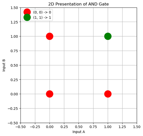
As you can see we have 4 data points and two categorical stand point in the plot, (0,0) , (0,1) , (1,0) and finally (1,1). As the AND gate logic goes, every input combination will result in a “zero” or a False output until the two inputs were “ones” and then the output changed to “one” or a True.
Let’s say we want to create a computational model to do the work of an AND gate by creating a decision boundary in our plot.
It seems so easy as the data points are separable linearly.
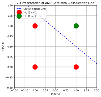
The plot will show the data points (0,0), (0,1), (1,0), and (1,1) with the decision boundary learned by the model. Points are color-coded based on their true class, and the decision boundary separates the 0 class from the 1 class.
But what if we have more complex data in a more complex space? How the model will learn then?
We can’t just separate the data points with a linear line! That’s where the “Activation Functions” come into play.
For example, lets plot an XOR gate:
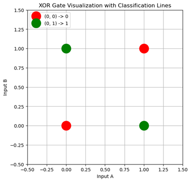
Here we need some non-linear function to correctly map data and separate the classes.
The activation function in an artificial neural network (ANN) plays a critical role in determining the output of a neuron. It introduces non-linearity into the model, which is essential for the network to learn and model complex patterns.
Here’s why the activation function is crucial:
1. Introducing Non-Linearity
Without an activation function, a neural network would be simply a linear combination of inputs and weights. No matter how many layers the network has, the entire network would act as a single linear transformation. This means the model could only learn linear relationships between inputs and outputs.
Activation functions like ReLU, Sigmoid, and Tanh introduce non-linearities, enabling the network to learn complex patterns, interactions, and representations in the data.
2. Enabling Multi-Layer Networks
In multi-layer networks (deep networks), activation functions allow each layer to learn different levels of abstraction. For example, early layers might learn simple features like edges in an image, while deeper layers learn more complex patterns like shapes or even object parts.
Without non-linear activation functions, these layers would collapse into a single layer with no added benefit from having multiple layers.
3. Thresholding and Decision-Making
Some activation functions, like the sigmoid, squash the output to a range (0 to 1), which can be interpreted as probabilities. This is particularly useful in classification tasks.
Activation functions like ReLU set negative values to zero, allowing networks to decide which neurons should be “active” or “inactive,” effectively creating a sparse representation and improving computational efficiency.
4. Gradient-Based Learning
Activation functions like Sigmoid and Tanh are differentiable, meaning that their derivatives can be used in backpropagation to update the network’s weights during training.
While ReLU has a non-linear derivative, it is still simple and effective for gradient-based optimization. The choice of activation function affects how gradients flow through the network and how efficiently the network can be trained.
5. Enabling Complex Decision Boundaries
Activation functions allow neural networks to form complex, non-linear decision boundaries. This is essential for solving real-world problems like image recognition, natural language processing, and other tasks where simple linear models are insufficient.
Sigmoid
Among these functions, the ”Sigmoid Function“ is one of the most well-known and widely used for classification tasks. In this post, we’ll dive into the magic of the sigmoid function, why it’s used, its strengths and weaknesses, and when to consider alternatives.
The sigmoid function is especially valuable in binary classification tasks, where we predict between two classes (e.g., yes/no, 0/1). By mapping the output of a model to a value between 0 and 1, the sigmoid function allows us to interpret that output as a probability of belonging to a particular class. Values closer to 1 indicate a higher probability of being in class 1, while values closer to 0 suggest class 0.
Sigmoid:


Here, ( e ) (Euler’s Number) is approximately 2.718 and is a constant in mathematics, essential for modeling exponential growth and decay. This exponential nature helps create a smooth curve, which is crucial for gradient-based optimization.
The sigmoid function as we can see is an s-shaped curve. For any value of x the sigmoid function will output a value between 0 and 1.
As said before, sigmoid function which is denoted by the Greek letter Sigma is given as 1 over 1 plus the exponential of minus X.
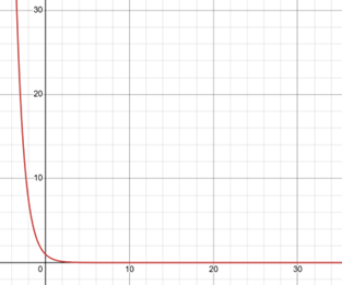
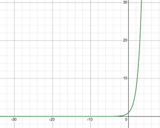
Here the exponential of minus X is the inverse of the well-known exponential function how does the plot of the inverse of the exponential look like let us plot both exponential(green) and it’s inverse(red) on the same graph
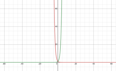
the inverse of the exponential has the same profile as the exponential function the only difference is the inverse exponential is flipped with respect to the y-axis if we study the limits of the inverse of the exponential function, we can see that when X takes large negative values toward minus infinity the infests exponential diverges to plus infinity.
Characteristics of the Sigmoid Function:
- Output Range: The sigmoid function maps any input x to an output value between 0 and 1. This makes it useful for models that need to predict probabilities, as the output can be interpreted as a probability.
- Smooth Gradient: The sigmoid function has a smooth gradient, which helps in the learning process during backpropagation. The function’s derivative is continuous and non-zero, ensuring that small changes in input result in small changes in output.
- Non-Linear: The sigmoid function introduces non-linearity into the network, enabling it to learn and model complex patterns. Without non-linearity, the network would only be able to represent linear functions, regardless of how many layers it has.
One interesting property of the sigmoid function is that it effectively compresses inputs within a narrow range, roughly between -5 and 5. Beyond this range, the function approaches either 0 or 1 so closely that any further changes in x make a negligible difference. For example, any input less than -5 will produce an output very close to 0, and any input greater than 5 will be near 1.
When we look at the sigmoid function graph, it has a characteristic S-shape. This curve quickly rises from 0 to 1 as x increases, but only within a specific range. Outside this range, the curve flattens out. Here’s how it works:
- Middle Range Sensitivity (Approximately -5 to 5):
- Between approximately -5 and 5, the sigmoid function is highly sensitive to changes in x.
- Small changes in x within this range produce noticeable changes in the output.
- Saturation Beyond -5 and 5:
- When x is less than -5, the exponential term grows very large (since x is negative and the exponent flips the sign), causing the denominator to also grow. This results in a very small output close to 0, no matter how much further x decreases.
- Conversely, when x is greater than 5, the exponential term becomes very small because x is positive, making the denominator close to 1. As a result, the output is close to 1, regardless of further increases in x.
This compression property makes sigmoid useful for models that require output in a [0, 1] range, especially for binary classification. For each input, the sigmoid function provides an interpretable probability-like output, indicating the likelihood of a sample belonging to a specific class.
While sigmoid can work well as an output activation in binary classification, it’s generally not recommended for hidden layers in deep networks. The main reason is the vanishing gradient problem. In regions where the function outputs values close to 0 or 1, the gradient (or slope) is very small. During backpropagation, this tiny gradient slows down or even stops the learning process, especially in deep networks, which need more robust gradients for efficient learning.
(The vanishing gradient problem is the main reason sigmoid isn’t widely used in hidden layers. The small gradients in the function’s “flat” regions (i.e., where it approaches 0 or 1) can slow down or even stop the training process. This issue is especially problematic for deep networks, which rely on strong gradients to propagate error signals effectively. Additionally, the sigmoid function tends to saturate for large positive or negative inputs, further slowing the learning process.)
Sigmoid as a “Biased Average” Function
Another interesting interpretation of the sigmoid function is as a type of biased average. When combining multiple inputs, the sigmoid function acts like a smoothing filter, effectively reducing extreme values. This makes it particularly useful when a network requires a smoothed or averaged output, though this same smoothing can be detrimental in hidden layers.
For instance:
import numpy as np
def sig(x):
 return 1/(1 + np.exp(-x))


x = 1.0
print('Applying Sigmoid Activation on (%.1f) gives %.1f' % (x, sig(x)))

x = -10.0
print('Applying Sigmoid Activation on (%.1f) gives %.1f' % (x, sig(x)))

x = 0.0
print('Applying Sigmoid Activation on (%.1f) gives %.1f' % (x, sig(x)))

x = 15.0
print('Applying Sigmoid Activation on (%.1f) gives %.1f' % (x, sig(x)))

x = -2.0
print('Applying Sigmoid Activation on (%.1f) gives %.1f' % (x, sig(x)))output:
Applying Sigmoid Activation on (1.0) gives 0.7
Applying Sigmoid Activation on (-10.0) gives 0.0
Applying Sigmoid Activation on (0.0) gives 0.5
Applying Sigmoid Activation on (15.0) gives 1.0
Applying Sigmoid Activation on (-2.0) gives 0.1
Sigmoid Derivative and Its Role in Machine Learning
The derivative of the sigmoid function as an activation function is essential for backpropagation in neural networks, as it helps compute the gradient for updating weights. The sigmoid derivative’s shape ensures that the gradient remains between 0 and 0.25, which can make training slower. It’s part of why alternative activation functions like ReLU are often preferred for hidden layers in deeper networks.
Sigmoid derivatives:
σ′(x)=σ(x)⋅(1−σ(x))
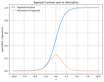
This formula indicates that the derivative (or slope) of the sigmoid function depends directly on the output of the sigmoid function itself.
Gradient Magnitude and the Vanishing Gradient Problem:
- In backpropagation, gradients are calculated based on the derivative of the activation function at each neuron. When using the sigmoid activation function, the gradients are always between 0 and 0.25.
- This narrow range of gradients means that weight updates are inherently small. When the output of a neuron is close to 0 or 1 (the “saturated” regions of the sigmoid curve), the derivative becomes very close to 0, leading to extremely small gradients.
- This results in the vanishing gradient problem: as gradients become very small, weight updates diminish, and training becomes slower. In deep networks, where many layers are stacked, this problem compounds as gradients are multiplied through each layer, often causing them to shrink to near-zero values for the earlier layers.
Effect on Learning Speed:
- Because the gradient is limited to 0.25 at most, the weight updates are constrained, making the learning process slower, especially when dealing with deep networks.
- This is particularly problematic in complex tasks that require a network to learn a large number of parameters. The network may take many more epochs (iterations over the training data) to converge to an optimal solution or may fail to converge effectively at all.
Solution to the vanishing gradient problem: A Hint at the Hyperbolic Tangent (Tanh) Function
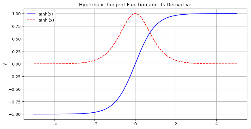
For hidden layers, the hyperbolic tangent (tanh) function is often preferred over sigmoid. Tanh is similar to sigmoid but ranges between -1 and 1, allowing for a broader range of values and helping with gradient propagation. In many cases, tanh can be a better choice as it doesn’t suffer from the same level of vanishing gradient issues, making it a powerful alternative.
Code:

Author:
Saman Chitsazian


