In the world of deep learning, the ADAM optimizer stands out as a reliable choice, celebrated for its efficiency and effectiveness in training complex models. But what makes ADAM so powerful? In this article, we’ll unpack ADAM’s foundations, from the basics of optimization to advanced techniques like exponentially weighted averages and RMSProp. By understanding these components, you’ll get a clearer picture of why ADAM is a top choice for training deep networks.
Optimizers: The Backbone of Model Training
Every machine learning model needs an optimizer to adjust its parameters, such as weights and biases, to minimize a loss function, which measures how well the model’s predictions align with actual outcomes. Different optimizers use unique algorithms to make these adjustments, aiming to find a balance between speed, accuracy, and computational efficiency. Optimizers like ADAM aim to achieve fast and stable convergence while effectively navigating complex data structures.
Gradient Descent: The Core Algorithm
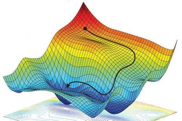
The foundation of optimization in machine learning is Gradient Descent (GD), a simple yet powerful method for minimizing loss functions. Imagine standing on a hill and wanting to get to the lowest point. Gradient descent takes small, calculated steps downhill by computing the gradient (slope) at each point.

In gradient descent, each step updates the parameters in the direction of the steepest descent based on the gradient:

where:
θ represents the parameters (weights and biases) being updated,
α is the learning rate, controlling step size, and
∇θJ (θ) is the gradient of the loss function with respect to θ.
While gradient descent is effective, calculating the gradient for each point in large datasets can be time-consuming and computationally expensive. Stochastic Gradient Descent (SGD) offers a faster, approximate approach.
Stochastic Gradient Descent: A Faster Alternative
Stochastic Gradient Descent (SGD) updates the model parameters by calculating the gradient for a single data point or a small batch at each step, rather than for the entire dataset. This approach introduces randomness in each update, adding noise to the optimization path. While this may seem like a drawback, the noise can help the optimizer escape from local minima, making SGD particularly useful for large, complex datasets.
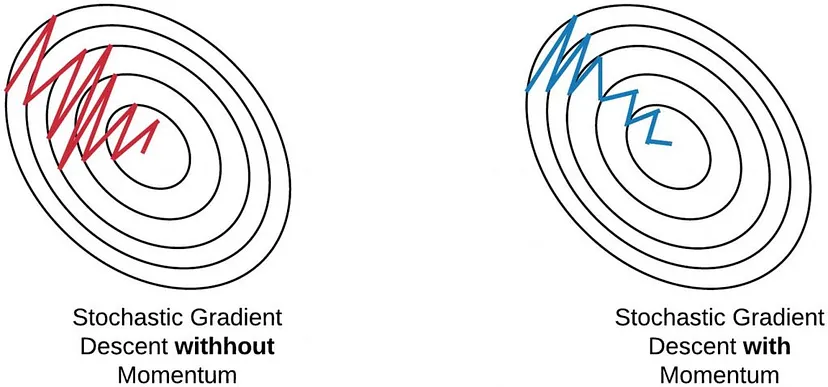
However, the noise in SGD can cause unstable updates, slowing down convergence. To counter this, techniques like Exponentially Weighted Averages and Momentum can smooth the updates, enhancing stability.
Exponentially Weighted Averages: Smoothing the Updates
Exponentially Weighted Averages reduce noise by calculating a smoothed version of the gradients. In this technique, each gradient update contributes to a moving average, with recent gradients carrying more weight than older ones.
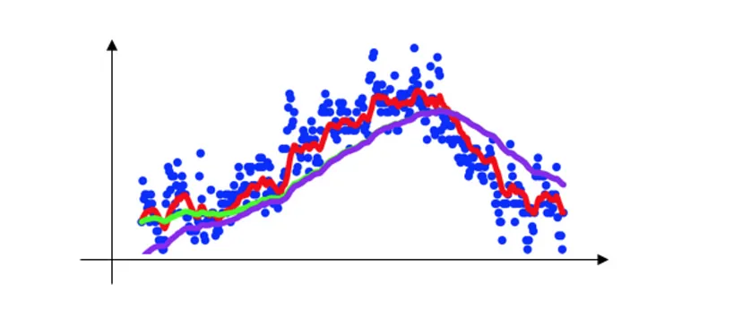
The formula for an exponentially weighted average at time t is:

where:
gt is the gradient at time t,
vt is the exponentially weighted average at t, and
β (between 0 and 1) controls the rate of decay.
Example: Let’s assume we have gradient values over four steps as follows: 3, 4, −2, 1. If we set β = 0.9, the weighted averages become:
1. Step 1: v1 = 0.9 × 0 + 0.1 × 3 = 0.3
2. Step 2: v2 = 0.9 × 0.3 + 0.1 × 4 = 0.67
3. Step 3: v3 = 0.9 × 0.67 + 0.1 × (−2) = 0.403
4. Step 4: v4 = 0.9 × 0.403 + 0.1 × 1 = 0.4627
This smoothed gradient sequence stabilizes the updates, which reduces oscillations and helps in converging more efficiently.
Momentum: Adding Velocity to Gradient Descent
Momentum builds on exponentially weighted averages by adding a fraction of the previous gradient to the current update, creating a “momentum” effect that propels the model faster in the optimal direction. This is similar to how a ball rolling down a hill gains speed as it moves. The formula is:
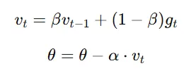
This approach makes gradient descent more effective at escaping local minima and moving faster in regions where gradients are flatter.
RMSProp: Adapting the Learning Rate for Stability
RMSProp (Root Mean Square Propagation) is another technique designed to improve gradient descent by adapting the learning rate for each parameter.
RMSProp uses Exponentially Weighted Averages to adapt the learning rate for each parameter dynamically, ensuring stable convergence. Although RMSProp itself doesn’t directly include a momentum term, its functionality is similar to momentum because it effectively smooths and stabilizes parameter updates by scaling them according to the history of past squared gradients.
RMSProp maintains a moving average of squared gradients, which helps balance the magnitude of updates across parameters. This is especially useful for optimizing complex models with many layers.
The RMSProp formula is:
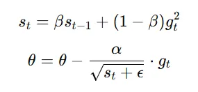
where:
st is the exponentially weighted average of squared gradients,
β controls decay,
α is the learning rate
ϵ is a small constant added for numerical stability
Example: Suppose we have squared gradient values over four steps: 9, 16, 4, 1, and we set β = 0.9 and ϵ = 10−8.
1. Step 1: s1 = 0.9 × 0 + 0.1 × 9 = 0.9
2. Step 2: s2 = 0.9 × 0.9 + 0.1 × 16 = 2.41
3. Step 3: s3 = 0.9 × 2.41 + 0.1 × 4 = 2.57
4. Step 4: s4 = 0.9 × 2.57 + 0.1 × 1 = 2.413
This gradually changing update size stabilizes the optimization process, especially for noisy datasets.
The ADAM Optimizer: Combining Momentum and Adaptive Learning
The ADAM optimizer (short for Adaptive Moment Estimation) combines the advantages of both momentum and RMSProp, offering adaptive learning rates with added stability. Here’s how ADAM works:
- Momentum component: ADAM keeps an exponentially weighted average of past gradients, helping retain the direction of optimal updates.
- Adaptive learning rates: ADAM also calculates an exponentially weighted average of squared gradients (similar to RMSProp), enabling it to adapt the learning rate for each parameter.
The parameter update rule for ADAM is as follows:
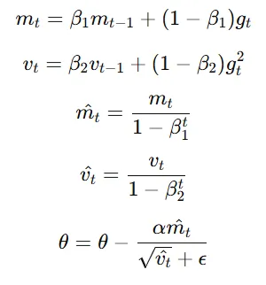
where:
mt and vt are the moving averages of gradients and squared gradients, respectively,
β1 and β2 control the decay rates,
m^t and v^t are bias-corrected estimates, and
α is the learning rate.
Why ADAM?
ADAM’s ability to adapt learning rates for each parameter combined with momentum allows for a faster and more stable convergence, especially for deep networks on large datasets. ADAM’s reliable convergence has made it popular among researchers and developers for optimizing deep neural networks, from simple image classifiers to cutting-edge language models.

Conclusion
The ADAM optimizer, as we’ve explored, is more than just an enhancement of gradient descent — it’s a sophisticated tool that incorporates momentum and adaptive learning rates to make deep learning models more effective. Understanding these components offers insight into why ADAM has become such a powerful tool for researchers and practitioners alike. Whether you’re a beginner or an experienced practitioner, mastering ADAM and its underlying principles is essential for effective and efficient model training.
